Understanding DeFi Yield Strategies used by AbraFi

For decades, investors have been accustomed to a binary choice: leave capital in “safe” bank savings accounts with minimal returns, or pursue higher growth in volatile markets. Yield-bearing stablecoins represent a modern shift in this paradigm, aiming to offer the stability of a dollar-pegged asset with the dynamic performance of decentralized finance (DeFi).

But how do these protocols actually generate yield without exposing the principal to the wild swings of the crypto market? The answer lies in sophisticated, automated “yield engines”— explore how these mathematical strategies operate 24/7 to capture market inefficiencies, and understand the investment concepts and mechanisms underlying these strategies. 

Using the AbraFi ecosystem as a model, here is an explainer on the four primary strategies that power AbraFi’s yield. The yield engines include:

1. Delta-Zero (liquidity-provision hedging)
2. Rho-Point (stable looping)
3. Theta-Flow (basis trades)
4. Sigma-Path (yield aggregation) 

Delta-Zero

The core market-neutral engine, this strategy leverages liquidity provision hedging. It seeks liquidity pools that provide substantial rewards on assets that have enough liquidity depth to mitigate high volatility inventory risk. 

At its core, this engine identifies opportunities to drive two simultaneous actions to seek return opportunities.

1. Providing liquidity to a market (earning fees by buying and selling an asset).

2. Hedging the inventory risk (using derivatives or offsetting positions to protect against sharp price movements in that asset).

How the Strategy Works

1. Providing Liquidity

The engine deploys assets into a market to facilitate external trading.

• Example: The system provides $100,000 worth of Liquidity to an ETH/USDC pool. This results in a “long” ETH exposure for a portion of the position.

2. Identifying the Delta (Exposure)

The engine calculates net exposure to the volatile asset (ETH). If the system’s liquidity position results in a 25 ETH long exposure, the delta is identified as +25.

3. Executing the Hedge

To neutralize that +25 delta, the system executes an offsetting short position with a delta of -25. This can be done via:

• Perpetual Futures: Shorting ETH perps on an exchange.
• Options: Buying put options to protect against a downside crash.
• Borrowing and Selling: Borrowing ETH from a lending protocol and selling it for stablecoins immediately.

4. Rebalancing

As the market moves, exposure changes. If the price of ETH rises, an AMM will automatically sell ETH for USDC, lowering the long exposure. The proprietary software dynamically adjusts the short position to maintain a substantially hedged position. This is called dynamic delta hedging.

Scenario Comparison: Hedged vs. Unhedged

Imagine you provide liquidity, and the price of the underlying asset drops by 20%.

Feature	Unhedged Liquidity Provision	Hedged Liquidity Provision
Fee Revenue	Earned consistently	Earned consistently
Inventory Value	Drops significantly	Drops, but offset by short position gains
Net Outcome	Net Loss (Fees < Asset Depreciation)	Illustrative Outcome (Fees earned, delta is flat)

Actual results may differ significantly from the examples shown.

Rho-Point

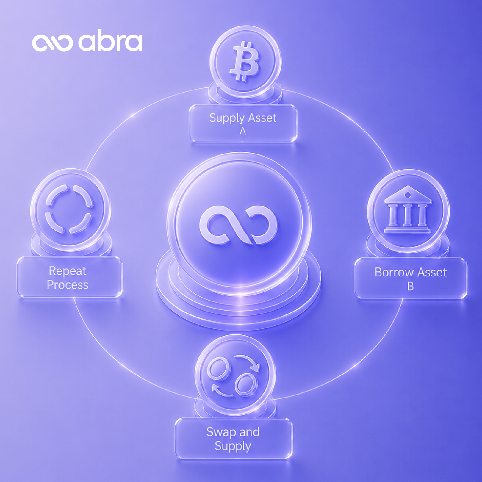
This yield engine uses leveraged staking (also referred to as stable-looping, or yield-looping) to add leverage to stable assets (USDC/USDT) or assets that maintain close parody (ETH/stETH). It’s often referred to as a form of arbitrage focusing on the yield the asset generates versus the cost to borrow it. Rho-Point identifies where these arbitrage opportunities exist and helps to seek enhanced return opportunities through leveraged exposure while employing risk-management techniques.

How the Strategy Works (The “Loop”)

The core idea is to deposit an asset, borrow against it, swap the borrowed asset back into the original asset, and deposit it again. This creates a leveraged position that multiplies your exposure to the yield.

Here is exactly how the strategy plays out using a stablecoin-to-stablecoin loop.

In this scenario, we will use USDT (Tether) and USDC (USD Coin). This type of looping relies on the fact that different stablecoins often have slightly different supply and borrow interest rates on major lending platforms like Aave or Morpho.

The Example: USDT / USDC Looping

Imagine the system is initialized with $10,000 in USDC and seeks to maximize yield without exposing the position to volatile assets like Bitcoin or Ethereum.

1. Deposit (Supply)

The strategy identifies a DeFi lending market where high demand from traders to borrow USDT results in a high interest rate for depositors.

• The engine deposits the initial $10,000 USDC as collateral.
• Let’s say the USDC Supply APY is 5.5%.

2. Borrow

Because USDC is used to borrow another stablecoin (USDT), the lending protocol considers this incredibly low risk. They allow for a high Loan-to-Value (LTV) ratio (often up to 90% to 95% in specialized “efficiency modes”).

• The system borrows $9,000 worth of USDT against the $10,000 USDC collateral (90% LTV).
• The cost to borrow USDT is 4.0% APY.

3. Swap & Loop

The system takes the $9,000 of borrowed USDT, executes a swap on a decentralized exchange (like Uniswap) back into USDC (paying a tiny trading fee).

The engine then deposits that $9,000 of fresh USDC back into the lending protocol.

• Total deposited collateral is now: $19,000 (earning 5.5%)
• Your total borrowed debt is now: $9,000 (costing 4.0%)

You can repeat this loop multiple times. If you execute this loop 4 or 5 times, your final position might look like this:

• Total USDC Collateral: $40,000
• Total USDT Debt: $30,000
• Initial capital deployed: Still just the original $10,000.

The Profit Math

Instead of capturing interest on just the initial $10,000, the system captures an interest rate spread across a much larger, leveraged position.

{Earnings from Collateral} = $40,000 *  5.5% = $2,200 /year

{Cost of Debt} = $30,000 *4.0% = $1,200 / year

{Net Profit} = $2,200 – $1,200 = $1,000 /year

By leveraging stablecoins through looping, the net return is $1,000 on the original $10,000 investment. Under the assumptions used in this hypothetical example, leveraged exposure may increase potential returns from a baseline of 5.5% to what is now 10%. Hypothetical illustration only. Actual results will vary and may result in losses.

Theta-Flow

This engine minimizes directional risk to seek exposure to basis spreads. This strategy captures the spread between spot and perpetual prices. The engine automates positions to support long spot, short perp — this produces a market-neutral strategy that harvests structural premiums. The strategy can generate significant yield in bull markets and a more compressed yield in bear markets where premiums also become less substantial.

How it Works: Step-by-Step Example on Bitcoin

Let’s say Bitcoin ($BTC$) is trading in a bullish market. Because traders are greedy and want to leverage up, they are willing to pay a premium to buy futures contracts.

1. The Setup

• Spot Price (S): $100,000
• Futures Price (F) (Expiring in 3 months): $104,000
• The Basis: $4,000 (a 4% premium for 3 months, or ~16% annualized)

2. Executing the Strategy

To seek to capture the basis spread, the strategy deploys $100,000 of capital:

1. Buy Spot: The engine executes a $100,000 buy to get exactly $100k of  BTC on the spot market.
2. Short Futures: The engine simultaneously opens a short position on of BTC using the 3-month futures contract at $104,000.

The strategy is now delta-neutral. Let’s see what happens at expiration under two different market scenarios.

3. The Outcome at Expiration

On the day the futures contract expires, the futures price and spot price must converge to the exact same value.

Scenario A: The Market Skyrockets (BTC goes to $150,000)

• Spot Profit/Loss: The strategy bought at $100,000 and it’s now worth $150,000. Profit = +$50,000
• Futures Profit/Loss: The strategy shorted at $104,000 and it’s now $150,000. Loss = -$46,000
• Net Return: $50,000 – $46,000 = $4,000

Scenario B: The Market Crashes (BTC drops to $60,000)

• Spot Profit/Loss: The strategy bought at $100,000 and it’s now worth $60,000. Loss = -$40,000
• Futures Profit/Loss: The strategy shorted at $104,000 and it’s now $60,000. Profit = +$44,000
• Net Return: -$40,000 + $44,000 = $4,000

The Result

Under the assumptions used in this simplified example, the Theta-Flow engine would have produced an illustrative result of $4,000 on a $100,000 investment. The strategy generated a 4% yield in 3 months completely independent of market direction.

Sigma-Path

This engine identifies opportunities for yield aggregation across lending markets and vaults to identify opportunities that may offer attractive risk-adjusted characteristics. The engine handles dynamic rebalancing across protocols and chains to seek to maintain a target risk profile.

Sharpe Ratio Explained

Developed by Nobel laureate William F. Sharpe, the ratio measures the excess return earned per unit of volatility. Historical Sharpe ratios are not predictive of future outcomes.

The Formula

Sharpe Ratio = (R𝘱 – R𝑓)/ σ𝘱

Where:

• R𝘱: Expected or Historical Return (in DeFi, this is the Pool’s APY).
• R𝑓: Risk-Free Rate. In traditional finance, this is usually a U.S. Treasury bond yield. In DeFi, investors often use a highly stable baseline, like the yield on a premier stablecoin pool (e.g., Aave USDC) or Ethereum liquid staking yields (e.g., stETH).
• σ𝘱 (Sigma): Standard Deviation of the returns. This represents the asset’s volatility—how wildly the pool’s APY swings day-to-day.

How to Interpret It

• Below 1.0: Suboptimal. You aren’t getting paid enough for the volatility you are enduring.
• 1.0 to 1.99: Good/Acceptable.
• 2.0 to 2.99: Very good.
• 3.0 or higher: Excellent.

How Sigma Path Works

With thousands of pools to sort through, this yield engine sorts through empirically driven filters to reduce selection only to pools meeting strict risk requirements. These parameters account for factors varying from the size of pool, time of inception, count of participants, and of course the current yield. Sigma Path calculates Sharpe ratios for each pool on an ongoing basis and runs scripts to manage rebalancing and allocation in each pool dynamically. 

The end result is a blended yield that is diversified across multiple pools that meets the target risk criteria (typically aiming for a blended Sharpe ratio of over 2, which may indicate favorable historical risk-adjusted characteristics.).

Summary

Understanding these strategies is just the first step toward optimizing your portfolio. Whether you are interested in the specific mechanics of dynamic delta hedging or how Sigma Path can improve your risk-adjusted returns, our team is ready to provide deeper insights for educational purposes and general discussion.

Digital asset strategies involve substantial risk, including the possible loss of principal. The examples contained herein are hypothetical and intended solely to illustrate how certain investment concepts may operate under specified assumptions. Hypothetical illustrations do not reflect actual investment results and are not guarantees of future performance. Strategies involving derivatives, leverage, decentralized finance protocols, and lending activities involve additional risks, including market risk, counterparty risk, smart contract risk, liquidity risk, operational risk, and regulatory uncertainty. There can be no assurance that any strategy described herein will achieve its objectives or avoid losses. Past performance is not indicative of future results.